 NOAA Technical Memorandum ERL CMDL-10
Cooperative Institute for Research in Environmental Sciences University of Colorado Boulder, Colorado
James H. Butler
Stephen A. Montzka
Richard C. Myers
James W. Elkins
Climate Monitoring and Diagnostics Laboratory Boulder, Colorado July 1995
UNITED STATES DEPARTMENT OF COMMERCE
Ronald H. Brown
Secretary
D. James Baker
Under Secretary for Oceans and Atmosphere/Administrator
Environmental Research Laboratories
James L. Rasmussen
Director
Mention of a commercial company or product does not constitute
an endorsement by NOAA Environmental Research Laboratories. Use
for publicity or advertising purposes of information from this
publication concerning proprietary products or the tests of such
products is not authorized.
This government document is provided for downloading and for the sole purpose of personal viewing and printing. The content of this document is not classified in any way. However, we expect every user to exclusively use this document in its entirety and we do not authorize any alteration, partial distribution or the
use of parts of it in other publications, neither do we permit the commercial use of any of its content. For questions regarding the use of this document, contact the authors.
This document is for sale by the National Technical Information Service, 5285 Port Royal Road Springfield, VA 22061
	ABSTRACT
1. 	INTRODUCTION
2. 	THE CRUISES
2.1. 	BLAST I
2.2. 	BLAST II
3. 	METHODS
3.1. 	Mass Spectrometric Air and Surface Water Measurements
3.2. 	Measurements of Water Column Samples
3.3. 	Other Measurements
4. 	CALCULATIONS
4.1. 	Mole Fractions (Gravimetric Mixing Ratios)
4.2. 	Data Correction for Warming of the Equilibrator
4.3. 	Saturation Anomalies and Fluxes
4.4. 	Atmospheric Properties
4.5. 	Flux Terms
4.6. 	Lifetimes and Ozone Depletion Potential
5. 	RESULTS
5.1. 	Ancillary Data for Both Cruises
5.1.1. 	BLAST I
5.1.2. 	BLAST II
5.2. 	Air and Surface Water Measurements
5.2.1. 	CFC-11
5.2.2. 	Nitrous Oxide
5.2.3. 	Methyl Bromide
5.2.4. 	Other Methyl Halides
5.3. 	Subsurface Measurements During BLAST II
5.4. 	Flask Analyses
6. 	DISCUSSION
6.1. 	Discrepancies With Previous Studies
6.2. 	Relationships With CH3Cl and CH3I
6.3. 	Oceanic Sources and Sinks of Atmospheric CH3Br
6.4. 	Conclusions
7. 	REFERENCES
8. 	APPENDICES
8.1. 	List of Tables
8.2. 	List of Figures
8.3. 	Acknowledgments
8.4. 	Data
The Nitrous Oxide And Halocompounds (NOAH) division of NOAA/CMDL participated in two research cruises in 1994 for the Bromine Latitudinal Air/Sea Transect project. Frequently collected CH3Br data from these expeditions constitute the largest data set for oceanic CH3Br to date, and the first solid estimate of oceanic emission, production and degradation of the compound. Our conclusion from these studies is that the ocean is probably not a net source of CH3Br, but rather a net sink. Although CH3Br is both produced and consumed everywhere in the surface ocean, the rate of consumption exceeds that of production in most waters sampled. Exceptions were coastal and coastally influenced waters, which were typically supersaturated, and areas of open ocean upwelling, where CH3Br saturations were close to zero. About 80% of the oceans are undersaturated in CH3Br, representing a net annual sink of 8-22 Gg y-1.
In addition to conducting two research cruises, we investigated potential contamination effects from sampling flasks and potential analytical artifacts from GC/ECD systems, developed a calibration scale for atmospheric and oceanic CH3Br and a global, finite-increment model for more precisely estimating the partial lifetime of atmospheric CH3Br with respect to oceanic losses.
CH3Br data from the second cruise indicate that our conclusions from the first expedition were qualitatively and quantitatively accurate. The latter results give greater strength to the global extrapolations of the first data set. Our best estimate of the partial lifetime of atmospheric CH3Br with respect to oceanic losses is 2.7 (2.4-6.5) y. This range was derived from a 40 year, global data set of sea surface temperatures and windspeeds. Data from the two expeditions suggest a shorter lifetime of CH3Br on the order of 2.4 y. The difference between the two estimates is due to the high windspeeds encountered during the cruises. Our estimate of the atmospheric lifetime, based upon combined atmospheric and oceanic losses, is now 1.0-1.1 y, compared to earlier estimates of 1.82.1 y when the ocean was considered an insignificant sink and tropospheric OH concentrations were underestimated by 15%. The oceanic sink correspondingly lowers the ODP for CH3Br by about one-third.
Work on the sampling and analytical uncertainties has revealed significant problems with the measurement of CH3Br in flasks, which have been used historically for virtually all previous measurements of CH3Br in the atmosphere. Whereas results from the shipboard system were free of sample storage effects and both the shipboard and the laboratory-based GC/MS systems were free of problems with co-eluting compounds, our results in analyzing flasks from the first expedition show that CH3Br in flasks often is unstable and will increase or decrease with time. In addition, we found that results for CH3Br determined by GC/ECD can be compromised by some GC configurations.
The distribution, flux, and lifetime of numerous atmospheric trace gases are affected significantly by the chemistry and biology of the ocean. This is readily apparent with gases that undergo reactions in the marine boundary layer, but it also is true for some of the longer-lived gases that have been implicated in stratospheric ozone depletion and global warming.
Methyl bromide (CH3Br) is of particular interest because it is both produced and consumed in the ocean, thus allowing the ocean to act as a buffer for CH3Br in the atmosphere. This simultaneous production and consumption of atmospheric CH3Br suggests that the atmospheric lifetime of this gas is shorter than would be calculated from net emissions or net consumption [Butler, 1994]. Although earlier reports declared the ocean a net source of CH3Br [Singh et al., 1983, Khalil et al., 1993], they did not agree quantitatively, leaving the budget of atmospheric CH3Br unresolved. The issue remains controversial because of recent attempts to regulate and ultimately eliminate anthropogenic emissions [Copenhagen Amendments to Montreal Protocol, 1994]. CH3Br apparently is responsible for about 50% of the organic bromine that reaches the stratosphere, where it can destroy ozone much faster than chlorine.
The main objective of the two NOAA/CMDL Bromine Latitudinal Air/Sea Transect expeditions has been to resolve the discrepancy in previously reported data for oceanic CH3Br, and to extend our understanding of the distribution and cycling of CH3Br between the atmosphere and ocean. This was pursued by making frequent, shipboard measurements of CH3Br in the surface water and the marine atmosphere along the cruise tracks and by obtaining depth profiles of CH3Br at selected stations. Secondary objectives included obtaining atmospheric and surface water data for other methyl halides, most notably CH3Cl, CH3I, CH2Br2, and CHBr3.
For the first expedition (BLAST 94), a transit leg of the
World Ocean Circulation Experiment line P18 was selected because
it covered coastal waters, central oceanic gyres, and regions
of divergence and upwelling in both hemispheres, as well as two
different seasons, winter in the northern hemisphere (NH) and
summer in the southern hemisphere (SH). The second expedition
(BLAST II) covered a wide latitudinal range similar to
that of the first cruise, but in the Atlantic Ocean. Results from
these cruises together allowed us to evaluate a wider, hence,
more representative range of world oceans. Also, the second cruise
took place during two different seasons, fall in the NH and spring
in the SH.
Although expected to be the only cruise during 1994 and initially labeled BLAST 94, in this report we will refer to the first cruise as BLAST I and to the whole project as BLAST 94.
BLAST I started on 26 January 1994 out of Seattle, WA. The cruise track led offshore to Ocean Station P at about 44°N/130°W, returning into San Francisco for exchange of scientific personnel. From there, the ship took a great circle route to Ancud, Chile at 41°S, where it went into the inland passage of the Chilean west coast, a waterway between the mainland and numerous little islands (Figure 1). The waters of this narrow inland passage were brackish, influenced by continental fresh water inflow. The ship arrived in Chile, on 18 February 1994.
Work for BLAST I was conducted aboard the NOAA Ship Discoverer (Fig. 2), a 93 m research vessel with around 50 crew members and capacity for about 40 scientists. Maximum cruising speed was 15.5 knots in colder waters, about 14 knots in warm waters. Windspeed measurements were taken 29.9 m above the waterline, the ship's lift out of the water during a typical transit leg is less than 1 m. The route from Seattle to Punta Arenas was a transit leg for WOCE line P18, which was to begin in Punta Arenas. During transit, only 5 scientists were aboard the Discoverer, three of which were from CMDL.
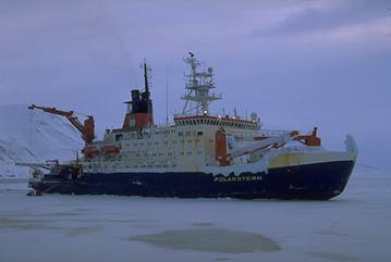
The second expedition started in Bremerhaven, Germany, on October 18, 1994, and was headed by the Alfred Wegener Institut (AWI). The first leg to Punta Arenas included a short (several hours) stop-over at San Miguel, Azores, at 38°N / 26°W for personnel exchange. After this, the ship stopped only for hydrocasts at spacings of 1-5° intervals. All sampling ceased at 47°S / 59°W because of an interdiction to sample in Argentine waters. This was just before reaching the continental shelf, which, at this point, extends quite far offshore. The cruise ended in Punta Arenas, Chile, on November 21, 1994.
The FS Polarstern is a 118 m long and 25 m wide research vessel, built and put into service exclusively for scientific purposes in 1982 (Fig. 3). Designed as an ice-breaker, the Polarstern is also equipped with stabilizers for smoother operation in rough waters. Normal cruising speed is 10-12 knots with a maximum of 16 knots. Windspeed measurements are taken 37 m above the waterline. The ship carries a crew of 41-44 members with a capacity for 50 scientists.
Our sampling approach allowed for frequent, automated, shipboard measurements of about 20 trace gases in the surface water and atmosphere with a gas chromatograph/mass spectrometer (GC/MS) (Table 1). Air for these measurements was sampled periodically from a continuous flow of 4-5 l min-1 from the bow; water was partitioned with a Weiss equilibrator [Weiss equilibrator] from which the circulating headspace was also sampled periodically [Butler et al., 1988, 1991a, Lobert et al., 1995b].
The GC/MS configuration was almost identical on both cruises [Lobert et al., 1995a]. About 200 ml of sample or calibration gas was trapped at 30 ml min-1 onto an Al2O3/KCl coated, megabore (0.53 mm ID) capillary at -50°C (Fig. 4b), with the sample flowing into a calibrated, evacuated volume. The sample was then transferred to the main column (0.25 mm ID x 30 m, DB-5; J&W) by flash heating (105°C, 3 min) of the trap. The HP5890A GC was connected to an HP5971 quadrupole mass spectrometer and temperature programmed to start at 20°C isothermal for four minutes, progress to 58°C at 15° min-1, then proceed to 220°C at 25°C min-1 and hold the final temperature for 3.4 minutes for a total runtime of 16.4 minutes. The oven was cooled with a Vortex tube (Vortec Corporation, Cincinnati), which was operated at 760 kPa of pressurized air delivered by the ship's compressors. Accounting for cooling time, samples can be injected at roughly 35 min intervals, alternating air and equilibrator (water) samples with two calibration gases. A typical chromatogram of an air sample is shown in Figure 4a.
| Compound Name | Formula | |||
| GC/MS system | ||||
| HCFC-22 | CHClF2 | |||
| HCFC-142b | C2H3ClF2 | |||
| Methyl Chloride | CH3Cl | |||
| CFC-114 | C2Cl2F4 symm | |||
| H-1211 | CBrClF2 | |||
| Methyl Bromide | CH3Br | |||
| Ethyl Chloride | C2H5Cl | |||
| CFC-11 | CCl3F | |||
| HCFC-141b | C2H3Cl2zF | |||
| Isoprene | H2C=C(CH3)CH=CH2 | |||
| Methyl Iodide | CH3I | |||
| CFC-113 | CCl3CF3 | |||
| Methylene chloride | CH2Cl2 | |||
| Methyl Nitrate | CH3ONO2 | |||
| ChloroBromoMethane | CH2BrCl | |||
| Chloroform | CHCl3 | |||
| Methyl Chloroform | CH3CCl3 | |||
| Benzene | C6H6 | |||
| Carbon Tetrachloride | CCl4 | |||
| DiBromoMethane | CH2Br2 | |||
| ChloroIodoMethane | CH2ICl | |||
| ChloroDiBromoMethane | CHBr2Cl | |||
| PerChloroEthylene | C2Cl4 | |||
| Bromoform | CHBr3 | |||
| DiIodoMethane | CH2I2 | |||
| GC/ECD system | ||||
| CFC-12 | CCl2F2 | . | ||
| CFC-11 | CCl3F | . | ||
| CFC-113 | CCl3CF3 | . | ||
| Methyl chloroform | CH3CCl3 | . | ||
| Carbon tetrachloride | CCl4 | . | ||
| Nitrous Oxide | N2O | . | ||
| Sulfur hexafluoride | SF6 | . | ||
During BLAST II, samples from hydrocasts were analyzed for dissolved N2O by an automated headspace sampling technique and GC/ECD [Butler and Elkins, 1991b]. Samples were collected at depth in 1-10 l Niskin bottles attached to a rosette capable of bearing 12-36 bottles. Hydrography was recorded with a conductivity-temperature-depth sensor (CTD) mounted at the center of the rosette. On this cruise, 24 samples and references could be analyzed for N2O within three hours, allowing us to keep up with hydrocasts at one degree latitude intervals.
Measurements of CH3Br, CH3Cl, and CFC-12 from Niskin samples on BLAST II were limited to hydrocasts at intervals of about four degrees latitude, because of the time required for the analyses. For these measurements, seawater samples were collected into 100 ml ground glass syringes directly from Niskin bottles. Initial attempts to collect dissolved CH3Br by a purge and trap technique proved faulty. Consequently, we elected to use a gas phase extraction technique [McAuliffe, 1971]. After sampling, half of the water in each syringe was displaced with ultra-high purity N2. The syringes were then shaken for 12 minutes with a mechanical wrist action shaker. The equilibrated headspace was injected through a Sicapent (P2O5) drying tube onto a packed Porapak Q trap (3.2mm OD stainless steel) at -45°C. After collection, this trap was rapidly heated to ~100°C, and the analytes desorbed and focused onto a second trap packed with Unibeads 1S at -45°C (1.6 mm OD, 0.5 mm ID). After the transfer, the focusing trap was heated rapidly to ~200°C, and the sample injected onto a Poraplot Q 0.53 mm fused silica column configured for backflushing (7 m precolumn, 14 m main column). The analytes were separated at 72°C and detected with an ECD at 350°C. CH3Br proved to be difficult to work with, owing mainly to contamination in the sampling system. Consequently, CH3Br data from some stations had to be discarded. Nevertheless, we were able to attain a number of reliable vertical profiles of CH3Br through the water column, with a sample repeatability on the order of 0.2 pM.
Measurements of gases other than CH3Br were necessary for this research. Gases that might be related in some way to the cycling of CH3Br (e.g., CH3Cl, CH3I) were obtained by GC/MS. We also needed information on advection and mixing in the ocean, for which some other gases are suitable tracers. The CFCs are conservative in seawater, i.e., under normal circumstances they do not react with seawater or any of its components and, hence, are good indicators for evaluating a variety of physical effects, such as those due to mixing or radiative heating. N2O is produced biologically at depth or in coastal sediments. It is present in surface waters only as a result of transport and mixing, hence is an excellent gas for identifying regions of upwelling or for defining the extent of coastal influence. Frequent measurements of 7 gases (Table 1) in the air and surface water were obtained with a custom-built, three channel electron capture gas chromatograph (GC/ECD). This system processes samples at 10 min intervals. The chromatography is isothermal with backflushed columns for high precision (0.2-2.0 %) analyses at short intervals [Lobert et al., 1995b, Elkins et al. 1996].
Samples of air and air equilibrated with seawater were collected into electropolished, stainless steel flasks on both cruises every five degrees in the higher latitudes and about every 2.5 degrees between 15°N and 10°S. The flasks were returned to Boulder for verification of shipboard measurements and for measurement of gases not obtained during the cruises. Supporting data for the ship's position and meteorological data for windspeed and direction, water and air temperatures, atmospheric pressure, humidity, and salinity of the surface water were continuously collected during both cruises. Those data were delivered by online systems of both ships and were interpolated to match the individual injections of both GC/MS and GC/ECD systems.
The dry atmospheric mole fractions of compounds from the GC/ECD system (e.g., CFC-11 and N2O) were determined as ratios of peak areas to those of two different standards injected before and after the sample. Assuming a linear response in the vicinity of the calibration gases (but a non-zero intercept of the response curve), we used the response factors of the two standards to compute mixing ratios for the samples by interpolating between them according to eq. 1.
 [1]
[1]where X and R refer to mole fraction and response and the subscripts S, 1, and 2 refer to sample, standard 1, and standard 2. Responses R1 and R2 for the standards were calculated from two points each, which were weighted according to their distance from the sample point. This 2-standard, 4-point method thus corrected for drift as well.
For all other measurements in this report, mole fractions were calculated with a one-point calibration (eq. 2). This approach is reasonable where the calibration curve is linear with an intercept equal or very close to zero, which applies to all of the GC/MS measurements made during these expeditions:
 [2]
[2]
Data from equilibrated seawater require a correction to account for warming of the water between the scientific sea water intake and the equilibrator. Water is warmed during transport because of insufficiently insulated tubing and exposure of the equilibrator to the sunlight on deck. Warming of the water results in elevated mixing ratios in the headspace of the equilibrator. This effect is small, but is easily corrected by computing a coefficient from the ratio of solubilities at two temperatures [e.g., Murphy et al., 1993; Butler et al., 1988]. Typical values for warming range from 0.01°C in warm waters to 0.8°C in cold waters.
Actual warming was calculated from both sea surface and equilibrator
temperatures, which were read from thermistors and recorded digitally
every minute during the cruise. For the final correction of equilibrator
data, we used solubility coefficients and their temperature dependences
listed in Table 2.
| . | ||||
35‰, 25° | ||||
(% deg-1) | ||||
(105 cm2 s-1) |
Certain anthropogenic gases, such as CH3CCl3 or CCl4, are consumed by reaction with seawater or by other processes. The partial atmospheric loss rates for these gases with respect to the ocean depend upon the aquatic degradation and air-sea exchange rates, and can be estimated from direct measurement of their partial pressures in air and water [Butler et al., 1991a, Lobert et al., 1995b].
At equilibrium, the partial pressures of inert halocarbons in the surface waters should be the same as they are in the atmosphere. Departures in partial pressure from theoretical equilibrium result from physical, chemical, or biological disturbances. For example, waters that have been warmed by solar radiation are generally supersaturated with the CFCs because gas evasion cannot keep pace with the rate of warming and the accompanying decrease in solubility [Kester, 1975]. Likewise, waters that have been cooled significantly can appear undersaturated with these gases. Air injection by bubbles from waves and whitecaps tends to supersaturate weakly soluble gases preferentially, and mixing of different water masses can lead to over- or undersaturations. Thus, departures of surface concentrations of non-reactive gases such as CFC-11 and CFC-12 from equilibrium are directly attributable to physical processes, and can be used to factor out physical effects for gases such as the methyl halides that are not conservative in seawater.
The saturation anomaly for a dissolved gas is defined as the percent departure of the observed dissolved amount from equilibrium. This is computed from the difference in partial pressures:
 [3]
[3]where pgw and pga are the partial pressures of the gas in water and air. If the saturation anomaly of a gas is positive, it indicates that the gas is leaving the water. If it is negative, then the gas is entering the ocean from the atmosphere. However, because of physical processes, the saturation anomaly alone is not sufficient for detecting or estimating in situ consumption or production in the water. The magnitude of physical effects depends upon the diffusivity of the gas, its solubility, and the temperature dependence of its solubility. In practice, the difference in saturation anomaly for similar compounds is small; saturation anomalies for CFC-11 and CFC-12 typically differ by only 13%. Their molecular diffusivities are not much different, nor is the temperature dependence of their solubilities, but their absolute solubility differs by a factor of 3.5. Although CFC-11 is not a perfect proxy for CH3Br, we estimate that it is more accurate to correct in part for physical effects rather than to ignore them completely.
Consequently, to determine if there is any loss of a gas in the water, we compute net saturation anomalies for all of the gases. For a tracer that is not too far out of equilibrium, the net saturation anomaly can be estimated by subtracting the CFC-11 saturation anomaly from the observed anomaly for each gas. Calculated this way, a net saturation anomaly that is negative indicates that the gas is probably being consumed in the water, regardless of its non-corrected anomaly. However, because of the differences in physical properties of various gases, net saturation anomalies smaller than ±2% are generally insignificant.
The net saturation anomaly should be roughly proportional to the in situ loss or production of the gas. If we assume steady-state conditions, the loss or production rate can be estimated from the flux of the gas across the surface of the water that is required to maintain the observed net saturation anomaly:
 [4]
[4]Here Fnet is the flux of the gas to the ocean (mol m-2 d-1), Kw is the air-sea transfer velocity (m d1), Hg is a modified Henry's Law constant for the gas (m3 atm mol-1) taken from Elliot and Rowland [1993], pga is the partial pressure of the gas in the atmosphere, g is the saturation anomaly of the gas and f is the saturation anomaly of CFC-11 (both in %). The flux of CH3Br across the air-sea interface, corrected for physical effects, should equal the sum of aquatic loss L and production P in surface waters. If we assume that f is adequate in correcting for physical effects, then, under steady-state conditions the net flux of CH3Br that is required to maintain the observed net saturation anomaly can be described by eq. 4. Consequently, aquatic degradation exceeds aquatic production where the net saturation anomaly is negative and vice versa. There is some uncertainty in this kind of flux estimate, mainly because Kw is known only to around 50% and varies considerably with wind speed and sea surface roughness. This introduces the biggest single uncertainty in our flux estimates, particularly because wind speeds during both cruises were very high. Also, the CFC-11 correction is only an approximation, as physical properties, such as solubility, are still somewhat different for both gases. For our estimates, Kw was calculated from Wanninkhof [1992].
 [5]
[5]where a is an empirically derived constant (0.47 for long-term winds, 0.37 for instantaneous winds, which was used in this report. ), u is the wind speed, and Sc is the Schmidt number, a dimensionless number defined as the kinematic viscosity of water divided by the molecular diffusivity of the gas in water at a given temperature. The constant 660 is the Schmidt number for carbon dioxide in seawater at 20°C. For our data, we derived the Schmidt number from diffusivities calculated from De Bruyn and Saltzman [1995], using sea surface temperature and wind speeds observed during the cruise.
The mean, dry, hemispheric mole fraction of CH3Br in the troposphere was determined with the following equation:
 [6]
[6]where is the hemispheric mole fraction in the troposphere, are the measured tropospheric mole fractions of the compound, and are the total number of moles in the troposphere and tropospheric hemisphere (ntr = 1.46 1020 moles [Warneck, 1988]), and i and I1 are the latitudes for each measurement, which define the beginning and the end of each incremental interval. For BLAST I, mixing ratios were assumed constant between 45.3°N and the North Pole (11.55 ppt) and between 53.3°S and the South Pole (8.25 ppt). Similarly, for BLAST II, mixing ratios were assumed constant between 48.7°N and the North Pole(11.5 ppt) and between 47.3°S and the South Pole (8.7 ppt).
Finally, the partial atmospheric lifetime with respect to oceanic loss, o, was computed from
 [7]
[7]with the area of the ocean A=361x1012 m2, the mean depth of the mixed surface water layer z=75m [Li et al., 1984], the reciprocal solubility Hg for each oceanic regime, the number of moles in the troposphere ntr, the fraction of CH3Br in the troposphere of 0.95 (derived from a vertical profile given in Lal et al., 1994) the air-sea exchange coefficient Kw, and the in situ degradation rate ks [Butler, 1994]. The term (kzDz)0.5 for downward removal is calculated from an in-situ degradation rate kz at an estimated thermocline temperature and the diffusivity Dz given by Li et al. [1984]. For practical purposes, the partial atmospheric lifetime of CH3Br was actually estimated as the sum of this computation carried out over small spatial increments, as the terms in the equation vary considerably over the ocean.
To better understand the behavior of non-conservative gases in the ocean, we have selected the following terms to label the origin and fate of methyl bromide illustrated in Figure 5.
The ocean is both a source and a sink for atmospheric CH3Br, as this compound is both produced and destroyed in the oceans (Fig. 5). Hence, source and sink terms should be viewed independently in budget calculations and lifetime estimates. In this manner, the treatment of CH3Br differs from that for gases that are only produced or only consumed in the ocean.
From published data about the loss L of CH3Br in the ocean owing to hydrolysis, nucleophilic chloride substitution [King et al., 1995], and downward removal [Butler, 1994], and from the net observed flux Fnet, calculated from saturation anomalies (eq. 4), we are able to estimate the total production P of the compound in seawater as the difference between the former two. The loss term enables us to calculate the partial atmospheric lifetime tauo of the compound due to oceanic removal (eq. 7). This lifetime, together with the mass of the troposphere of 1.461020 moles [Warneck, 1988], the fraction of CH3Br in the atmosphere that resides in the troposphere (0.95), and the partial pressure pa of the compound in the troposphere (eq. 6, corrected for water vapor; 10.1 ppt, Table 4), can be used to calculate the irreversible flux of CH3Br from the atmosphere to the ocean, labeled uptake:
 [8]
[8]About 60-75% of the CH3Br that is produced in seawater or enters the ocean from the atmosphere, is destroyed in the water (loss). Some of the CH3Br entering the ocean, however, returns to the atmosphere (return flux) and some of the CH3Br produced in the ocean is emitted to the atmosphere (emission). The fraction of CH3Br in the water that escapes to the atmosphere, whether it is derived originally from production or invasion, is defined by the term (1-R), where
 [9]
[9]is the fraction removed, ko is the pseudo-first-order rate constant for total degradation of CH3Br in the ocean (including downward removal), Kw is the air-sea transfer rate, and z is the mixed layer depth. The term, Kw/z, is the rate constant governing evasion to the atmosphere.
The total atmospheric lifetime of methyl bromide can be calculated by adding the inverse partial lifetimes with respect to removal by OH, stratospheric processes, ocean, and soils. Any additional sink for atmospheric CH3Br that might be found would need to be included into eq. 10.
 [10]
[10]Using this total lifetime enables us to provide a rough estimate of the ozone depletion potential (ODP) according to Mellouki et al. [1992] with
 [11]
[11]where the first quotient, equal to 1.08, denotes the ratio of Br release by CH3Br in the lower stratosphere relative to Cl release by CFC-11, and M, tau, and N are the molecular weight (g mol-1), the lifetime (y), and the number of halogen atoms in CH3Br. The factor alpha is the enhanced efficiency of bromine for ozone loss compared to CFC-11 (=48; WMO, 1995), and beta is a term to denote the distribution of the compound throughout the troposphere, which is equal to 1 for long-lived gases. MCFC-11, MCH3Br, tauCFC-11 are 137.37 g mol-1, 94.94 g mol-1, and 55 y, respectively. This approach is semi-empirical and strictly valid only for the lower polar stratosphere. It also includes the assumption of a well mixed distribution of the compound throughout the troposphere, hence, rather long lifetimes. The term beta in the above equation may actually be smaller than 1.0 for CH3Br (the value we used here) [Mellouki et al. 1992], as the compound turns out to be rather short lived.
Figure 6 displays some of the meteorological data obtained during this cruise. One major distinction from average meteorological data was the significantly higher true windspeeds during most of the cruise as compared to a long-term average wind field obtained from COADS data [Wright, 1988] (Fig. 6), with an average windspeed for the actual data set of 7.7 m s-1 compared to ~5.7 m s-1 for the average long-term wind field for this particular cruise track. For our air/sea exchange calculations, we used measured wind speeds (scaled to a height of 10 m) rather than an averaged wind field, assuming that observed surface water saturations of all compounds are defined by local winds. This assumption, however, is valid only if the actually observed wind speeds are representative for the short-term prevailing winds. In addition, windspeeds during this cruise were measured about 30 m above the waterline, making it necessary to scale them to a standardized 10 m height [Cardone et al., 1990].
A change in the true wind direction from ~80° to ~110° at 4.1°N denotes the interhemispheric tropical convergence zone (ITCZ). This feature is also evident in a change in atmospheric mixing ratios of some compounds that show a gradient between NH and SH. Winds were variable in the inland passage of Chile south of 41°S. The highest windspeeds observed during the cruise around 52°S coincided with a storm that developed towards the end of the cruise, which is also evident in the pressure data (Fig. 6).
Temperatures in both air and surface water (Fig. 6) are highest just north of the equator, with a distinct drop as the ship passed regions of equatorial upwelling at 1°S. Water temperature inside the equilibrator was 0.01 to 0.1°C warmer than the surface water temperature during this cruise, with slightly higher values in the inland passage and a distinct diurnal cycle throughout the tropics. Warming of the seawater en route to the equilibrator raises the partial pressure of gases by 3-5% per °C, an offset for which we corrected in our calulations. Warming is kept to a minimum by a high water flow rate of at least 60 l min-1, of which 20 l min-1 are passed through the equilibrator.
Surface water salinity dropped dramatically in the inland passage of Chile, where it is a measure of freshwater runoff (Fig. 6). The decrease in salinity of almost 50% within the passage suggests substantial freshwater dilution.
Windspeeds during BLAST II, averaging 8.4 m s-1, were even higher than those during the first cruise and deviated from the long-term mean mainly at 45°N, around the equator, and at 25°S to 30°S. The actual data (measured at 37 m above the sea surface and scaled to 10 m) do not show many features common to the averaged wind field, as was the case during BLAST I. A very sharp change in absolute wind direction from ~60° to ~210° at 6.4°N delimits the ITCZ, which, analogous to the first cruise, is observed in the air profiles of most of the compounds as a distinct change in mixing ratios. Trajectory analysis shows a very clear influence of NH air and SH air at 8°N and 5.5°S, respectively [Joyce Harris, NOAA/CMDL, personal communication].
Air temperatures during BLAST II were generally 1-2° lower than water temperatures until about 23°S, where air and water temperatures were roughly equal which is consistent with long-term averages from COADS.
Warming of water in the equilibrator was generally higher during this cruise, falling between 0.04°C in the tropics and 0.8°C near the end of the cruise. This was mainly caused by a 50 m long, uninsulated hose that was required for the positioning of the equilibrator on the stern.
Two low pressure systems were encountered at the beginning of the cruise and around 42°S, both of which caused air temperatures to drop. The second low pressure system also corresponds to a change in wind direction from north to west winds.
 Salinity drops distinctively between 12°N and 4°N, typical
for tropical oceanic regions, where precipitation exceeds evaporation,
and is highest in central gyres, where evaporation exceeds precipitation.
A slow gradient to lower salinity can be observed towards the
continents on either end of the plot as freshwater influence becomes
more apparent.
Salinity drops distinctively between 12°N and 4°N, typical
for tropical oceanic regions, where precipitation exceeds evaporation,
and is highest in central gyres, where evaporation exceeds precipitation.
A slow gradient to lower salinity can be observed towards the
continents on either end of the plot as freshwater influence becomes
more apparent.
During BLAST I, about 710 measurements of 20 compounds were obtained by GC/MS, about 250 each for air and surface water, plus about 2700 measurements of 7 gases obtained by GC/ECD, amounting to a total of 20000 signals for gases in air and surface water. Adding this to 2700 measurements of 7 gases obtained by GC/ECD, half of which were for air or surface water, yielded a total of 20000 signals for gases in air and surface water. N2O was sampled at 16 depths from 43 hydrocasts for a total of 688 analyses of dissolved N2O at depth. Profiles of CH3Br, CH3Cl, and CFC-12 were obtained from 14 of the hydrocasts taken along this transect.
Atmospheric mole fractions of CFC-11 decreased from north to south on both expeditions, which is typical for a reasonably long-lived, anthropogenic gas released primarily in the northern hemisphere. The mean mole fractions were 272.7 ppt and 266.9 ppt for the two hemispheres with a global mean of 269.6 ppt (Fig. 8) for the first cruise, and 270.3 ppt, 266.8 ppt, and 268.4 ppt, respectively, for the second cruise. The mixing ratios for both cruises in the southern hemisphere agreed fairly well, while northern hemispheric values dropped about 2.4 ppt. This is supported by a growth rate of CFC-11 that presently is close to zero or negative [Elkins et al., 1993] and an atmospheric mixing ratio that peaked during 1994 [NOAA/CMDL, unpublished data]. Accordingly, the interhemispheric difference dropped from about 5.8 ppt to 3.5 ppt during 1994. Partial pressures of CFC-11 in the surface water during both cruises were generally higher than in the air, causing a small supersaturation of 0-4% (Fig. 8), except in strong upwelling areas in the E. Pacific and near the coast of Chile during BLAST I, where CFC-11 depleted waters were brought up from depth. No such strong upwelling was observed during BLAST II.
Atmospheric mole fractions of nitrous oxide were 309-312 parts per billion (ppb) during the first cruise and 310-312 ppb during the second cruise. Slightly higher mole fractions in the NH during both cruises reflect a mean hemispheric difference of 0.5-1.0 ppb. Higher partial pressures of N2O in the surface water were associated with upwelling at the equator, at current divergences at about 10°N during BLAST I, and, in some instances, near the coast (50°N / BLAST II). N2O was also higher in coastal waters owing to continental runoff and, perhaps, influence of coastal sediments.
 Saturation anomalies of N2O were used to identify some
of the physiographical regions as delineated in Figure 1. Strong
upwelling signals from the equatorial East Pacific correlated
well with similar negative signals in the saturation anomaly of
CFC-11. Ultimately, these were used to denote physiographic regions
2, 3, and 4 of Figure 1. Regions 6 and 7 were assigned from the
saturation anomalies of CH3Br (Fig. 10) and the location
of the inland passage (41°S).
Saturation anomalies of N2O were used to identify some
of the physiographical regions as delineated in Figure 1. Strong
upwelling signals from the equatorial East Pacific correlated
well with similar negative signals in the saturation anomaly of
CFC-11. Ultimately, these were used to denote physiographic regions
2, 3, and 4 of Figure 1. Regions 6 and 7 were assigned from the
saturation anomalies of CH3Br (Fig. 10) and the location
of the inland passage (41°S).
On average, atmospheric CH3Br ranged from 11.5 ppt in the northern hemisphere to 9 ppt in the southern hemisphere, indicative of a global distribution of sources and sinks favoring greater emission in the northern hemisphere (Fig. 10 and 11; Table 4). The latitudinally weighted, global mean mixing ratio derived from both cruises, is 10.1 ppt. Data collected during the second cruise are more scattered because of greater uncertainty associated with the sensitivity of the GC/MS system. Also, the interhemispheric gradient during the second cruise was slightly weaker than during the first cruise (Table 4), because of a higher SH mean. This could be a seasonal effect and has to be investigated further. Although the SH mixing ratios were higher during the second cruise, the averaged NH/SH ratio remained at 1.3 with an interhemispheric difference of 2.5 ppt.
| . | estimate | ||
| Global mean (ppt) | 9.8 | 10.4 | 10.1 |
| NH mean (ppt) | 11.2 | 11.7 | 11.5 |
| SH mean (ppt) | 8.6 | 9.4 | 9.0 |
| IHD (ppt) | 2.65 | 2.31 | 2.48 |
| Uncertainty (ppt) | 0.6 | 1.2 | . |
| NH/SH ratio | 1.31 | 1.25 | 1.28 |
| ITCZ (°N) | 4.1 | 6.4 | . |
Both partial pressures in the surface water and saturation anomalies for CH3Br in the Atlantic (Fig. 11) followed a pattern similar to that observed in the East Pacific. During both cruises, the central gyres were 20-50% undersaturated in CH3Br, waters near the equator and open ocean upwelling were near equilibrium, and coastal waters or waters associated with the Humboldt current offshore of Chile and the Brazil current were supersaturated in CH3Br to levels as high as 100%. The locations of these latter two incidents are exceptions from the coastal water definition given in Kossina [1921] as the area between coast and 200 miles offshore. However, the saturation anomalies of methyl bromide in these areas were atypical for the remaining open ocean. As in both cases a current carrying waters from shore to the open ocean was involved, we decided to extend the definition for 'coastal' waters to 'coastal and coastally-influenced' waters.
The gap in CH3Br data near 21°S during BLAST II stems from a rise in both atmospheric mixing ratio and surface water partial pressure that could not be explained by any log entry, meteorological feature, or other reasonable cause, and that didn't show in any other compound. Flask analyses, which, for CH3Br, generally agreed with shipboard data, indicate that the rise in mixing ratios at this location, as suggested by our shipboard measurements, was not real (Fig. 11, round symbols). For these reasons, we removed the shipboard data between 19°S and 23°S from the BLAST II data set.
For global estimates, individual measurements were used to derive individual fluxes, which were combined into one data base, sorted by region, and averaged over the three main regions; these data are summarized in Tables 5 and 6. Table 5 lists sea surface temperatures and wind speeds (scaled to 10 m) averaged for both cruises and saturation anomalies for the individual and the combined cruises. There are some differences in CH3Br saturation anomalies between the two cruises. Whereas the open ocean values were roughly equal, saturations in both coastal and upwelling regions were significantly lower during the second cruise. Figure 11 shows an extended latitudinal area with positive saturation anomalies south of 30°S. However, these saturations were not nearly as high as those during the first cruise approaching the Chilean coast. Similarly, upwelling regions in the East Pacific were slightly supersaturated, in contrast to the undersaturated Atlantic upwelling regions.
(°C) |
(m/s) |
(%) BLAST I |
(%) BLAST II |
(%) combined |
|
| Open ocean {1, 5, 9, 12} | 23.6 | 6.8 | -24.6 | -23.4 | -23.9 |
| Coastal {2, 6, 8, 13} | 15.6 | 8.5 | 37.1 | 2.7 | 14.0 |
| Upwelling {3, 4, 10, 11} | 26.6 | 7.1 | 2.61 | -12.2 | -6.9 |
| Total | . | . | -15.71 | -19.71 | -18.4 |
If our definition of oceanic regions is representative for upwelling areas of the oceans, and saturation anomalies reflect productivity patterns determined by upwelled waters, the results would be consistent with the fact that upwelling typically is stronger in the E. Pacific than in the Atlantic Ocean. Finally, the global net saturation anomaly of -18.4% is not much different from our first estimate of 15.7% in Lobert et al [1995a], due to the predominance of the open ocean values.
Net fluxes, loss, and production of oceanic CH3Br are comparable for both cruises. Our new estimate of Fnet is about 10% more negative than the value published in Lobert et al. [1995a]. Values from Tables 5 and 6 for BLAST I differ from those published in Lobert et al. [1995a]. Those differences originate from using different equations for calculating the diffusivity [De Bruyn et al., 1995], solubility [Elliot and Rowland, 1993] and the total degradation rate for CH3Br in seawater [King et al., 1995] for this report. The equation of De Bruyn et al.for the diffusivity of CH3Br was preferred here over the one published by Hayduk and Laudie [1974], because it is based on actual measurements. Similarly, the solubility equation published by Elliot and Rowland is considered superior over the one published by Singh et al. [1983] because it is based on actual measurements in seawater, rather than in pure water with an applied salting-out coefficient. Also, the combined degradation rate for nucleophilic displacement by Cl- and neutral hydrolysis was recently measured by King et al. [1995] for smaller increments and for a more suitable range of temperatures (10-35°C) than was done by Elliot and Rowland [1993] (0 and 22C). Finally, the estimate of King et al. [1995], which includes both neutral hydrolysis and nucleophilic displacement, doesn't depend upon separate measurements of the hydrolysis rate in freshwater (e.g., Mabey and Mill [1978]).
The estimates of King et al. [1995] and Elliot and Rowland [1993] are very close. The difference in computed oceanic lifetime of CH3Br is only 0.4%. The difference between the solubilities of Elliot and Rowland [1993] and Singh [1983], however, is about 15%, which directly translates into a 15% lower partial lifetime estimate. The diffusivity terms of De Bruyn [1995] and Hayduk and Laudie [1974] differ by about 30%, which, in the combined BLAST data set, results in a 10% lower lifetime and a 10% larger Fnet. Finally, instead of using the mass of the entire atmosphere, in this report we use the mass of the troposphere divided by the fraction of CH3Br that resides in the troposphere (0.95) for calculating the lifetime of the compound. This results in a 13% lower lifetime of CH3Br with respect to oceanic removal. The last row in Table 6 contains data from Lobert et al. [1995a] treated the same way as the combined data set in this report.
| Region | factor |
(%) |
(m3 atm mol-1) |
(m d-1) |
(Gg y-1) |
(Gg y-1) |
(Gg y-1) |
(10-12 mol l-1 d-1) |
| Open ocean | 0.8 | -23.9% | 6.20 x10⁻³ | 4.6 | -182 | +167 | 0.222 | |
| Coastal | 0.1 | 14.0% | 4.62 x10⁻³ | 7.2 | -12.5 | +13.9 | 0.149 | |
| Upwelling | 0.1 | -6.9% | 6.84 x10⁻³ | 4.6 | -34.0 | +33.4 | 0.356 | |
| Global | . | -18.4% | 6.10 x10⁻³ | 4.9 | -229 | +214 | 0.228 | |
| BLAST I revised |
-15.7 |
5.85 x10⁻³ |
5.9 |
-188 |
175 |
0.187 |
||
| BLAST II | . | -18.57 | . | . | . | . | . | . |
The global net saturation anomaly was derived from weighting the numbers in row 1 to 3 with the weighting factor.
The row "BLAST I revised" contains data from Lobert et al [1995a] re-calculated the same way as the values in "Global"
Contrary to an earlier study [Singh et al., 1983, 1993], dissolved CH3Br did not correlate with dissolved CH3Cl. Both CH3Cl and also CH3I were highly supersaturated everywhere along both cruise tracks, hence, a correlation of surface water partial pressures of CH3Cl is not useful for directly predicting levels of oceanic CH3Br. A linear regression analysis of surface water partial pressures for the first cruise yields the following correlations between CH3Br, CH3Cl and CH3I
 [12]
[12]
 [13]
[13]Both CH3Cl and CH3I are unlikely to be useful for a practical prediction of CH3Br levels, as r2 would amount to only 0.003 and 0.04, respectively. Other methyl halides measured on both cruises include CH2Br2, CHBr3, CH3I, CH2I2, CH2ICl, and CHBr2Cl, all of which were moderately to highly supersaturated in surface waters.
CFC-12 decreased with depth below the mixed layer (50-200 m) at all stations, as would be expected for an inert tracer of atmospheric origin (Fig. 13). High quality CH3Br profiles were more difficult to obtain because of contamination problems, arising from a number of potential sources during sample storage and analysis (section 3.2.). CH3Br and CH3Cl profiles were obtained at 16 stations between 25°N and 44°S. CFC-12 was also measured to account for variability due to the purely physical processes of transport and mixing.
In general, surface concentrations ranged between 0.5 and 3.5 pM for CH3Br and between 60 and 275 pM for CH3Cl. To detect possible production or degradation, only the ratios of the peak area for each sample to the peak area for the surface sample are shown in Figure 13. The concentrations of all three species were higher within the mixed layer than at depth. This suggests that both CH3Br and CH3Cl have sources associated with surface waters because the only source for CFC-12 in the ocean is through uptake from the atmosphere.
If CH3Br and CH3Cl were conservative gases in seawater, their profiles, ratioed to the surface water concentration, would resemble that of CFC-12. Departures from the CFC-12 profile result from in situ production or degradation of the gas. For example, removal of CH3Br in the lower mixed layer is suggested in the second and third profile in Figure 13. Some of the departures of the CH3Br and CH3Cl profiles from those of CFC-12 within the mixed layer may be the result of biological processes. However, there are no supporting biological data from this cruise indicating which types of organisms were present at these depths. Further research is necessary to determine which organisms may be affecting the distribution of CH3Br in the water column.
Qualitatively, CH3Br and CH3Cl profiles are similar to those measured by Atlas et al. [1994]. However, the CH3Br concentrations in Atlas et al. [1994] are approximately 2 to 5 times higher than those observed during BLAST II, likely owing to the colder water near Antarctica, where the study of Atlas et al. [1994] was conducted. The degradation of CH3Br is much slower and solubility is higher at low temperatures.
Measurements of methyl bromide in flask samples were generally in good agreement with underway data (Fig. 10, 11). Results of repeated analysis of flasks from the first expedition, however, demonstrate that in some cases there is a significant trend in CH3Br mixing ratios with time (Fig. 14). This is most likely due to a surface effect inside certain canisters which is not understood at this time. We also demonstrated that at least one GC/ECD configuration (Al2O3 / KCl PLOT focusing trap and a non polar, methyl siloxane column; J&W DB-1) was capable of yielding artificially high values for CH3Br in flasks of air from the equilibrator. So high, that it gave the appearance of supersaturations where, in fact, undersaturations existed. GC/ECD measurements of CH3Br on a DB-1 column with a Poraplot-Q focusing trap, however, produced results identical to those by GC/MS; the same was observed for a GC/ECD equipped with Poraplot Q and Al2O3/KCl traps and a Poraplot Q column. A system similar to our GC/ECD/Poraplot Q setup (Scripps Institute of Oceanography), produced values that are in general agreement with our analyses (shaded area at ~270 days), The SIO values are slightly lower, because of a calibration scale for CH3Br that appears to be ~10% lower than CMDL's.
Only in three flasks, out of 15 that showed a CH3Br drift, was CH3Br decreasing, whereas it increased in the remaining 12 affected flasks. Not all flasks, however, were faulty. About 70% of all flasks agreed well with shipboard results (Fig. 10, 11) and appear to be reliable for sample storage. Still, our results show that flask analyses for CH3Br can be inaccurate by as much as 25% within one month after sampling (flask 4423, Fig. 14) if the canister reveals a trend in mixing ratios.
Our results, showing that most of the ocean is undersaturated in CH3Br and that the ocean is likely a net sink for this compound, contrast sharply with those of the two previous investigations of CH3Br in seawater. It is possible, however, that our results are not in direct conflict with those of Singh et al. [1983]. Neither of the BLAST cruises encountered tropical waters under coastal influence, where much of Singh's work took place. Our coastal measurements were all from temperate regions, where the saturation anomaly was large and positive and the water cooler. Thus, measurements of Singh et al. [1983] may, in part, represent the saturation anomaly for tropical, coastal waters. However, the cruise track they followed should have taken them into waters of the tropical, open ocean, where we observed the largest, negative saturation anomalies ( 50%). Further, the measurements were done by GC/ECD with a liquid phase analytical column similar to one that produced analytical artifacts in our laboratory. We have not directly tested Singh et al.'s [1983] column under identical circumstances for this effect. However, even if data of Singh et al. [1983] were correct, they would represent only a small part of the ocean and would be unlikely to reverse the estimated global oceanic flux of atmospheric CH3Br.
Although BLAST 94 data might be compatible with those of Singh et al. [1983], the difference between our findings and those of Khalil et al. [1993] cannot be reconciled by geographic variability. Both of the cruises, upon which samples of Khalil et al. [1993] were collected, crossed the Pacific Ocean from New Zealand to California, traversing coastal waters, central gyres, and current divergences. Results of Khalil et al. [1993] should have been similar to ours, but they were not.
During both of the BLAST 94 cruises, we collected marine air and air from the equilibrator into flasks similar or identical in make to those used by Khalil et al. [1993]. Our results, showing that CH3Br could increase or decrease significantly in the flasks within a month's time (Fig. 14), indicate that samples of Khalil et al. [1993] may not have been stable during the time between sampling and analysis, which apparently was on the order of months. Khalil et al. [1993] analyzed their samples by GC/ECD with a non-polar methyl-siloxane column, but we cannot tell if flasks of air from the equilibrator yielded artificially high results. Their trap was made of inert materials and different from the ones we tested in our laboratory.
To resolve the question of which system was yielding correct results, we looked carefully at both analytical approaches. In this study, flasks that were collected during the cruises were analyzed with a GC/MS in Boulder, which had a sample inlet, trap, and column configuration different from the shipboard system [Montzka, 1993]. This reduced the possibility of artifacts that might have been associated with our shipboard GC/MS. ECD signals, however, can be enhanced by co-eluting peaks, which, by themselves, may or may not yield a response on the ECD. In fact, doping an analytical system with small amounts of O2 or N2O is a common practice now used to enhance the signals of certain molecules [Grimsrud and Miller 1978, Elkins et al., 1996]. CO2 and CH4 both yield virtually no response on an ECD, but they can greatly enhance the ECD response to N2O [Phillips et al., 1979; Crill et al., 1995]. With this in mind, we scanned some flask samples, both with the shipboard GC/MS and the flask GC/MS, and found numerous hydrocarbons eluting near or with the CH3Br peak. These hydrocarbons were found in very large quantities in air from the equilibrator, but not in ambient air samples. Although not conclusive, this does raise suspicion over GC/ECD analyses for CH3Br with a non-polar, methyl silicone-coated column.
Finally,we analyzed some cruise flasks with a GC/ECD using a different column (0.53 mm ID 21 m Poraplot Q) for separation of peaks and by GC/ECD with a different (Poraplot Q) trap. The results obtained by these two GC/ECD systems were consistent with those obtained by GC/MS, thus strongly indicating that analyses of CH3Br in seawater samples on the one GC/ECD were flawed and that the analyses by GC/MS are correct.
These results suggest that the sampling and analysis of CH3Br in air and seawater is not trivial. Significant artifacts can arise when samples are stored for short periods, and analysis by GC/ECD can be problematic, particularly when the samples being analyzed originate from seawater. Sampling and analytical approaches that have worked well for numerous halocarbons may not all be suitable for the measurement of CH3Br. Any program involved in the measurement of CH3Br must include a careful evaluation of these potential effects.
Singh et al. [1983] reported that CH3Br and CH3Cl were highly correlated in their samples. This apparent correlation has led to the assumption that one could predict CH3Br concentrations in the ocean by extrapolating from CH3Cl distributions [UNEP, 1992; Singh and Kanakidou, 1993]. Our data, however, show that there is little if any similarity of CH3Br with CH3Cl or CH3I in the surface waters (Fig. 12). Further, our findings of a sink for atmospheric CH3Br over most of the ocean where there is clearly a source of CH3Cl, suggest that the processes regulating these two compounds are different and that, to a first degree, a correlation of concentrations should not be expected. This is readily apparent when one considers the importance of displacement of Br in CH3Br by Cl-, a process that does not affect the concentration of CH3Cl.
Data of Singh et al. [1983] represent a limited geographic area, but the real problem with the apparent correlation is with some outlying data points. The whole relationship is weighted heavily by one data point, and, without it and two more outliers, loses most of its significance.
Until recently, it was generally understood that the most probable lifetime for CH3Br in the atmosphere was around 2 y, due primarily to reaction with OH in the troposphere [Singh and Kankidou, 1993; UNEP, 1992]. The possibility of an oceanic sink was acknowledged, but was considered to be effective only in parts of the ocean that might be undersaturated [Singh and Kanakidou, 1993]. Because evidence at the time suggested that the ocean was highly supersaturated in CH3Br [Singh et al., 1983; Khalil et al., 1993], a strong oceanic sink was thus considered unlikely. However, the ocean operates as a sink everywhere and the lifetime of atmospheric CH3Br with respect to the ocean must be independent of the production and saturation of CH3Br [Butler, 1994]. The oceanic sink of atmospheric CH3Br depends mainly upon sea-surface temperature and the rate of air-sea exchange, not upon the saturation anomaly, which is simply a measure of simultaneous production and loss. Using globally weighted averages for critical variables in this relationship, Butler [1994] suggested that the atmospheric lifetime of CH3Br, including this oceanic sink, would drop from 1.8 y to 1.2 y. Regardless of this oceanic sink, the ocean was still believed to be a large net source of atmospheric CH3Br, i.e., losses to the ocean were thought to be outweighed by production and emission. From a study conducted offshore of the Americas, Singh et al. [1983] suggested that the mean saturation anomaly of CH3Br was 240% and estimated the net global oceanic source of CH3Br at 300 Gg y-1. From samples collected on two trans-Pacific research cruises, Khalil et al. [1993] suggested that the overall oceanic supersaturation was 40-80%, yielding a net global oceanic flux of 35 Gg y-1. Recognizing possible differences between sampling areas, Singh and Kanakidou [1993] revised the estimates of Singh et al. [1983] to account for the limited geographic coverage of the data set, settling on a value for the net oceanic flux of CH3Br to the atmosphere of 60 Gg y-1.
Our research effort was initiated to resolve the difference between the two existing studies, and to provide an additional estimate for the magnitude of CH3Br. As described earlier, this study was designed to sample different oceanic regimes and to eliminate potential artifacts associated with sampling and analysis. By covering large sections of the open ocean and including upwelling and coastal regions in both hemispheres of two oceans and in four seasons, the lack of adequate and representative global coverage was curtailed. Problems associated with sampling and storage were obviated by making shipboard measurements, and potential ECD-specific artifacts were eliminated by using a GC/MS. Further, the relatively frequent analyses during these two cruises yielded highly robust data sets that are by far the largest collection of data on oceanic CH3Br to date. Because of the care taken in calibration, sampling, and analysis, we believe it to be accurate and free of significant artifacts. Results from the two cruises show that most of the ocean is not a net source of atmospheric CH3Br, but rather a net sink.
Data from the Pacific cruise suggested a global net sink of about 13 Gg y-1. The combined estimate from both cruises suggests a net sink of 15 Gg y-1. This net flux of CH3Br from the atmosphere into the ocean contrasts strongly with the findings of Singh et al. [1983] and Khalil et al. [1993]. Our findings further highlight a problem in an earlier perception of the budget of atmospheric CH3Br. This is simply the need to consider all sources and sinks of atmospheric CH3Br separately, including those from the ocean. Invoking a net oceanic flux in budget calculations can be misleading and, in the case of lifetime calculations, incorrect [Butler, 1994]. Properly, one should think of aquatic production, aquatic loss, oceanic emission to the atmosphere, and oceanic uptake from the atmosphere as separate terms in the budget (Fig. 5). For example, data from both cruises combined now suggest that global aquatic production and loss are 214 and 229 Gg y-1, while emissions and uptake between the ocean and atmosphere are 45 and 60 Gg y-1, respectively. If, for some reason, the atmospheric burden, and hence, the atmospheric partial pressure, of CH3Br drops, the amount of CH3Br taken up by the ocean at the new steady state (uptake) will have decreased and the amount emitted (emission) will have remained the same. This increases the net flux from the ocean, but does not alter the atmospheric lifetime of CH3Br with respect to the ocean, which was estimated to be 2.4 years according to eq. 7 using the combined data set. The lifetime given in Lobert et al. [1995a], modified with the change in terms mentioned in 5.2.3., would be 2.5 years. Both of these lifetimes agree within their uncertainty, but are at the low end of the range of possible lifetimes given in Yvon and Butler [1996] of 2.4 to 6.5 years. Yvon and Butler [1996] used a coupled, ocean-atmosphere box model and a 40 year, tightly gridded data set of oceanic and atmospheric properties from Wright [1993] to derive their range and a best estimate of 2.7 y.
The main reasons for the low value from the BLAST 94 measurements
are the higher wind speeds observed on both cruises as compared
to the long-term COADS wind field in Wright [1988]. As mentioned
earlier, windspeeds, averaged over the entire cruises, were 7.7
and 8.9 m s1. This represents a 35% and
27% departure from the COADS data for the same cruise tracks that
average at about 5.7 and 6.6 m s-1. The median value
for the combined data set is 7.72 m s-1 compared to
a locally weighted, global mean of 6.5 m s-1 in Yvon
and Butler [1996], representing a ratio of 0.85. If the individual,
observed windspeeds in our data set are multiplied with 0.85,
the combined, best lifetime estimate would change from 2.4 to
3.0 years, still as close to the value of Yvon and Butler [1996]
as the unadjusted value, but now well within their range of possible
lifetimes. This clearly demonstrates that the single most sensitive
input into our calculations, and, hence, the single largest uncertainty,
is the air-sea exchange coefficient Kw according
to eq. 5. It also indicates that actually observed winds might
not be suitable for global estimates.
| Source | |
| Butler [1994] | |
| Lobert et al. [1995a] | |
| Lobert et al. [1995a], revised | |
| Combined data set from both cruises | |
| Combined data set (adjusted to COADS) | |
| Yvon and Butler [1996]; current best estimate |
Prinn et al. [1995] recently revised the ALE/GAGE calibration scale for CH3CCl3, yielding a value that is about 18% lower than their previous estimate, which has been the historical basis for calculations of atmospheric OH. Their new calibration scale is now within 6% of the calibrations of NOAA/CMDL, suggesting that the new value is probably the more accurate one. Regarding CH3Br, this has the effect of lowering its lifetime with respect to atmospheric removal from 2.0 y to 1.67 y. Another manuscript by Shorter et al. [1995], identifies a previously unreported soil sink for atmospheric CH3Br of 42+/-32 y, which, in combination with our atmospheric values, would represent a partial atmospheric lifetime of 3.4 y. This study is more tentative, in that it is the only one of its kind, but the authors conducted their tests in the laboratory and field for a number of different soil types. The value is highly uncertain, but, because the atmospheric lifetime would now be computed from the inverse lifetimes of three separate sinks, the uncertainty is greatly reduced in the final estimate of the total lifetime.
Based on the lifetime of 2.7 y for oceanic degradation from Yvon and Butler, [1996], a partial lifetime of 1.67 y for atmospheric removal including stratospheric losses [Prinn et al., 1995], we can calculate a total lifetime for atmospheric CH3Br of 1.03 y by adding the inverse single lifetimes according to eq. 10. This estimate is about half of the earlier used estimate of 1.8-2.1 y, which was based on atmospheric removal alone and an underestimate of the mean tropospheric OH concentration. Adding the results of Shorter et al. [1995] of 3.4 y for breakdown in soils, we estimate an even lower total lifetime of 0.8 y, with a possible range including all known uncertainties of 0.6 y to 1.3 y [Yvon and Butler, 1996].
This revised lifetime estimate would reduce the ozone depletion potential (ODP) according to eq. 11 from 0.6 [WMO, 1995] to 0.4, with a possible full range of 0.3 to 0.6.
Our perception of the budget of atmospheric CH3Br has changed considerably within the past two years. Much of this is reflected in the recent Scientific Assessment of Ozone Depletion: 1994 [WMO, 1995], although some of the information there is now in need of revision. Specifically, the oceanic source, as listed in WMO [1995], is estimated at 60-160 Gg y-1, based mainly upon the data of Khalil et al. [1993] and the review of Singh and Kanakidou [1993]. Data from this report show that the oceanic source is more likely on the order of 45 Gg y-1, unless there is a large, hitherto unidentified, polar source. This new estimate places a tighter constraint upon the budget of atmospheric CH3Br, in that greater emissions from other sources are required.
The large uncertainties in the air/sea exchange coefficient affect computation of both oceanic emissions and uptake of atmospheric CH3Br. Refining the estimate of this term can shorten the range of the lifetime estimate, but its greatest impact will be upon the estimate of oceanic emissions which are directly related to the exchange rate with the atmosphere. Thus, the error in Kw in this instance translates directly to the same relative error in oceanic emissions. Improvement in our understanding of the term will certainly enhance the ability to quantify the oceanic source.
The bigger uncertanties with regard to the budget of atmospheric CH3Br now lie with the sources. The data from BLAST 94 suggest an oceanic source much smaller than that given in the WMO [1995] report. Nevertheless, the two cruises, for all of the area they covered, did not encompass tropical coastal waters, nor the warmer waters of the W. Pacific Ocean, nor the unique waters of the Indian Ocean with their extensive subsurface anoxic zones, nor cold, polar and subpolar waters. Although additional studies of these regions will not affect the calculated partial atmospheric lifetime of CH3Br with respect to oceanic loss, such investigations would be useful in refining and narrowing the range of the estimated oceanic source of CH3Br.
Anbar, A.D., Y.L. Yung, and F.P. Chavez.
Atlas, E., R.Lueb, S. Madronich, B. Prezlin, and R. Smith.
Butler, J.H., J.W. Elkins, C.M. Brunson, K.B. Egan, T.M. Thompson,
T.J. Conway, and B.D. Hall.
Butler, J.H., J.W. Elkins, T.M. Thompson, and B.D. Hall.
Butler, J.H., and J.W. Elkins.
Butler, J.H.
Cardone, V.J., J.G. Greenwood, and M.A. Cane.
Crill, P.M., J.H. Butler, D.J. Cooper, and P.C. Novelli.
Copenhagen Amendment to the Montreal Protocol.
De Bruyn, W.J. and E.S. Saltzman.
Elkins, J.W. T.M. Thompson, T.H. Swanson, J.H. Butler, B.D. Hall,
S.O. Cummings, D.A. Fisher, and A.G. Raffo.
Elkins, J.W., D.W. Fahey, J.M. Gilligan, G.S. Dutton, T.J. Baring,
C.M. Volk, R.E. Dunn, R.C. Myers, S.A. Montzka, P.R. Wamsley,
A.H. Hayden, J.H. Butler, T.M. Thompson, T.H. Swanson, E.J. Dlugokencky,
P.C. Novelli, D.F. Hurst, J.M. Lobert, S.J. Ciciora, R.J. McLaughlin,
T.L. Thompson, R.H. Winkler, P.J. Fraser, L.P. Steele, M.P. Lucarelli.
Elliot, S. and F.S. Rowland
Phillips, M.P., R.E. Sievers, P.D. Goldan, W.C. Kuster, F.C. Fehsenfeld.
Grimsrud, E.P, D.A. Miller.
Hayduk, W. and H. Laudie.
Kester, D.R.
Khalil, M.A.K., R.A. Rasmussen, and R. Gunawardena.
King, D.B., C. Pilinis, and E.S. Saltzman.
Kossina, E.
Lal, S., R. Borchers, P. Fabian, P.K. Patra, and B.H. Subraraya
Li, Y.-H., T.-H. Peng, W.S. Broecker, H.G. Östlund,
Lobert, J.M., J.H. Butler, S.A. Montzka, L.S. Geller, R.C. Myers,
and J.W. Elkins.
Lobert, J.M., J.H. Butler, T.J. Baring, R.C. Myers, S.A. Montzka,
and J.W. Elkins.
Mabey, W. and T. Mill.
McAuliffe, C.
Mellouki, A., R.K. Talukdar, A.-M. Schmoltner, T. Gierczak, M.J.
Mills, S. Solomon, and A.R. Ravishankara.
Montzka, S.A., R.C. Myers, J.H. Butler, and J.W. Elkins.
Murphy, P.P., C. Cosca, D.C. Lee, and R.A. Feely
Pilinis, C., D.B. King, and E.S.Saltzman.
Prinn, R.G., R.F. Weiss, B.R. Miller, J. Huang, F.N. Alyea, D.M.
Cunnold, P.B. Fraser, D.E. Hartley, and P.G. Simmons.
Ryther, J.H.
Shorter, J.H., C.E. Kolb, P.M. Crill, R.A. Kerwin, R.W. Talbot,
M.E. Hines, and R.C. Harriss.
Singh, H.B., L.J. Salas, and R.E. Stiles.
Singh, H.B. and M. Kanakidou.
UNEP, 1992. D.L. Albritton and R.T Watson.
Wanninkhof, R.
Warneck, P.
Warner, M.J., and R.F. Weiss
Weiss, R.F. and B.A. Price.
Weiss equilibrator
WMO
Wright, P.B.
Yvon, S.A. and J.H. Butler
Table 1: Gases measured continuously during the two cruises
Table 2: Some physical data for all compounds
Table 3: Flux terms and their derivations
Table 4: Atmospheric data for CH3Br from both cruises
Table 5: Observed values for CH3Br in three main marine regions
Table 6: Calculated coefficients and fluxes for CH3Br in three main marine regions
Table 7: Partial lifetimes of CH3Br with respect to oceanic loss
Figure 1: Cruise tracks for the two BLAST cruises
Figure 2: NOAA Ship Discoverer
Figure 3: FS Polarstern
Figure 4a: Air sample chromatogram
Figure 4b: Schematic of the GC/MS system
Figure 5: Schematic of CH3Br cycling between the oceans and the atmosphere
Figure 6: Ancillary data for BLAST I
Figure 7: Ancillary data for BLAST II
Figure 8: CFC-11 for both cruises
Figure 9: N2O for both cruises
Figure 10: CH3Br for BLAST I
Figure 11: CH3Br for BLAST II
Figure 12: CH3Br versus CH3Cl and versus CH3I
Figure 13: Depth profiles for CH3Br, CH3Cl, and CFC-12
Figure 14: Results from analyses of flasks taken during BLAST I
We thank the captains and crew of both the NOAA Ship Discoverer and the F.S. Polarstern for their cooperation and assistance during these expeditions, and are grateful to NOAA/PMEL and AWI for providing the opportunities. We also would like to thank Joyce Harris for trajectory analysis and Matt R. Nowick for his electrical expertise before and during the BLAST I expedition. This work was funded by the Methyl Bromide Global Coalition under contract number CTR 93-2, the Atmospheric Chemistry Project of NOAA's Climate and Global Change Research Program, and an appointment to the Global Change Distinguished Postdoctoral Fellowships sponsored by the U.S. Department of Energy, Office of Health and Environmental Research, and administered by the Oak Ridge Institute for Science and Education.
Data from this report, other published data from the Nitrous Oxide and Halocompounds (NOAH) division, some online publications, as well as graphs and mission logos are available through a public account on our UNIX server. To download these data, use your FTP (file transfer protocol) communications utility. Connect to ftp://ftp.cmdl.noaa.gov/noah/ocean/, logon with username anonymous and use your email address yourname@email.net as your password. See the directory structure below (as of February 1996) for locating the BLAST data. Once logged on, please make sure to view the file "readme1st.txt" before you download data. In most cases, you do not need to download all files, but rather a few files that are specific for your needs. Set your system to binary transfer by typing binary or clicking on the "binary" checkbox. Please refer download- questions and problems to Thayne Thompson at tthompson@cmdl.noaa.gov or call our secretary at +1 303 497 6811. You can get more convenient access to both data and publications through our World Wide Web (WWW) homepage at http://www.cmdl.noaa.gov/noah_home/noah.html. Select "data" or "publications" from the menu. We recommend using an HTML 3.0 capable browser.